- Details
- Written by: Steve Burgess
One question I’ve been asked a large number of times is how to perform a power calculation in Mendelian randomization for a binary exposure. We wrote a longer paper on the difficulties of MR with a binary exposure previously (Mendelian randomization with a binary exposure variable: interpretation and presentation of causal estimates), but we removed details on power calculation due to limited word count.
The short answer is that it's not simple, and potentially not possible unless you have additional data. If the gene—exposure associations are estimated on the odds ratio scale, it makes a big difference to power if the exposure is rare (e.g. for an odds ratio of 1.2, the genetic variant would increase exposure prevalence from 0.1% to 0.12% in absolute terms) or the exposure is common (e.g. the genetic variant increases exposure prevalence from 10% to 12%). Power depends on the absolute magnitude of the increase in the exposure prevalence, not the relative increase on the odds ratio scale. So if you have no way of estimating genetic associations with the exposure on an absolute scale (such as linear regression of the exposure on the genetic variant), then you can't calculate power.
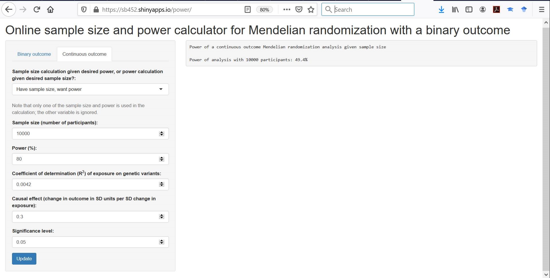
If you can get the IV—exposure associations on an absolute scale (e.g. the genetic variant increases the prevalence of the outcome by 2% - say from 10% to 12%), then you can calculate power. But power calculations are still not simple as power is normally given for a proposed effect size per 1-SD unit increase in the exposure, and a 1-SD change for a binary exposure may be a little difficult to conceptualize. Instead, we can consider the proposed per 1 unit increase in the exposure (from 0 to 1). In this case, you can use standard tools for power calculation (such as Online sample size and power calculator for Mendelian randomization with a binary outcome), but instead of the R^2 measure, you need a different value. This is obtained by taking the beta-coefficient from linear regression of the exposure on the genetic variant (call this number beta). For a biallelic SNP, instead of the R^2 statistic, you want beta^2*2*MAF*(1-MAF).
So if you have a genetic variant that is a SNP with a minor allele frequency of 0.3 that increases the prevalence of the exposure by 10%, then your replacement “R^2 value” is 0.1^2*2*0.3*0.7 = 0.0042. Power to detect a 0.3 SD increase in the outcome per 1 unit increase in the exposure in a sample size of 10,000 would be around 50%, as shown in the screenshot below:
A quick simulation exercise demonstrates that this value is fairly accurate:
set.seed(496)
times = 1000
parts = 10000
pval = NULL
for (j in 1:times) {
g = rbinom(parts, 2, 0.3)
x = rbinom(parts, 1, 0.2+0.1*g)
y = rnorm(parts, 0.3*x)
pval[j] = summary(lm(y~g))$coef[2,4]
}
sum(pval<0.05)
> [1] 492
Hope that is helpful!
- Details
- Written by: Steve Burgess
Given the global situation with reduced travel and face-to-face content, it is not possible to plan an in-person course in the foreseeable future. So, the November 2020 version of the Mendelian randomization course will be delivered remotely via an online learning platform. We are currently working through details of how this will work - please be patient and bear with us while we work through the details!
UPDATE: Course is now full! We are hoping to repeat in Spring 2021.
- Details
- Written by: Steve Burgess
Recently the PhenoScanner webtool has been updated by James Staley and colleagues (in particular Mihir Kamat). A number of factors were improved in the update, including more genetic associations, and the ability to search associations by gene and by risk factor. Another important update is that PhenoScanner can now be called directly from R. Here we present some code demonstrating how to call PhenoScanner from R, and how to integrate output from the PhenoScanner package into the Mendelian randomization package, and perform Mendelian randomization using a single line of R code.
Please note that this code is currently inefficient, as the PhenoScanner code currently queries the whole database, rather than specifically querying just the desired variables. Watch this space for developments! However, this does mean that the code may run slowly, particularly if many people across the world are trying to access the resource simultaneously.
The first step is to install the PhenoScanner package (and the MendelianRandomization package if you haven't done this previously):
install.packages("devtools")
library(devtools)
install_github("phenoscanner/phenoscanner")
library(phenoscanner)
install.packages("MendelianRandomization")
library(MendelianRandomization)
The code below takes as inputs a list of rsids, the name of the exposure (risk factor), the PubMed ID of the study that published the association estimates for the exposure, and the ancestry group for the association estimates (eg "Mixed", "European", or "African") - this triple of name/PubMed ID/ancestry is required to uniquely specify a dataset for genetic associations - and the name, PubMed ID and ancestry group for genetic associations with the outcome. It creates an MRInput object, which can then be used as an input for the functions in the MendelianRandomization package.
pheno_input <- function(snps, exposure, pmidE, ancestryE, outcome, pmidO, ancestryO) {
dataTable <- phenoscanner(snpquery = snps, pvalue = 1)$results
snp.list.exposure = unique(dataTable[which(dataTable$trait == exposure & dataTable$pmid == pmidE & dataTable$ancestry == ancestryE & !is.na(dataTable$beta) & !is.na(dataTable$se)),1])
snp.list.outcome = unique(dataTable[which(dataTable$trait == outcome & dataTable$pmid == pmidO & dataTable$ancestry == ancestryO & !is.na(dataTable$beta) & !is.na(dataTable$se)),1])
snp.list = intersect(snp.list.exposure, snp.list.outcome)
if (length(snp.list) == 0) { cat("No variants found with beta-coefficients and standard errors for given risk factor and outcome combination. Please check spelling and PMIDs.\n"); return() }
row.exp = NULL; row.out = NULL
for (j in 1:length(snp.list)) {
row.exp[j] = which(dataTable$trait == exposure & dataTable$pmid == pmidE & dataTable$ancestry == ancestryE & !is.na(dataTable$beta) & !is.na(dataTable$se) & dataTable$snp == snp.list[j])[1]
row.out[j] = which(dataTable$trait == outcome & dataTable$pmid == pmidO & dataTable$ancestry == ancestryO & !is.na(dataTable$beta) & !is.na(dataTable$se) & dataTable$snp == snp.list[j])[1]
}
Bx. <- dataTable[row.exp, c("snp", "beta", "se")]
By. <- dataTable[row.out, c("snp", "beta", "se")]
dataSet <- merge(Bx., By., "snp")
return(mr_input(exposure = exposure, outcome = outcome, snps = as.character(dataSet[,1]),
bx=as.numeric(dataSet[,2]), bxse=as.numeric(dataSet[,3]), by=as.numeric(dataSet[,4]), byse=as.numeric(dataSet[,5]),
correlation = matrix()))
}
pheno_obj = pheno_input(snps=c("rs12916", "rs2479409", "rs217434", "rs1367117", "rs4299376", "rs629301", "rs4420638", "rs6511720"),
exposure = "Low density lipoprotein", pmidE = "24097068", ancestryE = "European",
outcome = "Coronary artery disease", pmidO = "26343387", ancestryO = "Mixed")
This code can then be combined with any of the functions from the MendelianRandomization package to perform a Mendelian randomization analysis. Here, we use the mr_ivw function to perform a Mendelian randomization analysis in a single line of R code:
mr_obj = mr_ivw(pheno_input(snps=c("rs12916", "rs2479409", "rs217434", "rs1367117", "rs4299376", "rs629301", "rs4420638", "rs6511720"),
exposure = "Low density lipoprotein", pmidE = "24097068", ancestryE = "European",
outcome = "Coronary artery disease", pmidO = "26343387", ancestryO = "Mixed"))
This analysis shows that LDL-cholesterol is a causal risk factor for coronary artery disease, with an estimate of 0.498 corresponding to an odds ratio of exp(0.498) = 1.65 per 1 unit (here, one standard deviation) increase in LDL-cholesterol.
Comments are welcome!
- Details
- Written by: Steve Burgess
The MendelianRandomization R package was recently updated to version v0.2.2. There were some fixes in terms of p-values and confidence intervals (for example, previously p-values were based on a t-distribution regardless of the choice specified by the user). The package can be downloaded from https://cran.r-project.org/web/packages/MendelianRandomization/index.html. A paper introducing the package can be found at https://www.ncbi.nlm.nih.gov/pubmed/28398548.
- Details
- Written by: Steve Burgess
MR Catalogue (http://mrcatalogue.medschl.cam.ac.uk/), a web-based tool for performing genetic look-ups in publicly-available data, was launched today. The tool takes genetic variants (either rsid or chromosome and position) as inputs, and outputs the associations of the variants (batch query is needed for multiple variants) with up to 200 different variables, including disease outcomes and continuous phenotypes. There is an option for a proxy search, so that if your specified variant is not available, the association of a correlated variant will be given. The default display is the top 10 associations (ranked by p-value); a download is needed to access all associations. Genetic associations (including proxies) have been orientated across datasets, so that the signs of all association estimates are consistent.
This tool enables Mendelian randomization to be performed quickly and easily using summarized data - beta-coefficients and standard errors - see http://www.ncbi.nlm.nih.gov/pubmed/24114802, http://www.ncbi.nlm.nih.gov/pubmed/25773750, or http://spark.rstudio.com/sb452/summarized/ for details on how to perform a basic Mendelian randomization analysis using summarized data, or http://www.ncbi.nlm.nih.gov/pubmed/26050253 (MR-Egger) https://www.academia.edu/15479132/Consistent (median-based method) for robust methods using summarized data.
Outside of Mendelian randomization, this is a useful tool for calculating proxies, or checking the association of variants with a wide range of variables (phenome scan). Even if you switch off the catalogue and the proxy search, it is a quick tool for converting chromosome/position (hg19) to rsid and vice versa, or for getting major/minor alleles. Hopefully will be a widely used tool!